After twenty years managing fabric production and quality for global brands, I've seen more disputes over tolerance specifications than any other single issue. Last quarter, a promising partnership between an American retailer and Chinese mill collapsed over a 3% GSM variance that technically fell within the purchase order's vague "commercial quality" tolerance—but rendered the fabric unusable for their automated cutting equipment. The problem wasn't the mill's capability but the mismatch between stated tolerances and actual production requirements.
Setting appropriate tolerances requires balancing technical feasibility with commercial requirements. Too tight, and you'll face supply shortages and premium pricing; too loose, and you'll receive unusable product. Through developing tolerance standards for brands ranging from luxury houses to mass retailers, we've established that optimal tolerances depend on fabric type, manufacturing technology, and end-use requirements rather than one-size-fits-all standards.
Establishing effective tolerances requires understanding five critical aspects: technical feasibility based on manufacturing capabilities, commercial implications of acceptance/rejection decisions, testing methodology impacts on measured values, end-use sensitivity to variations, and relationship management implications. Let me guide you through our systematic tolerance-setting methodology.
What technical factors determine feasible GSM tolerances?
GSM (grams per square meter) tolerance setting must account for raw material variability, manufacturing process control capabilities, and testing method precision. The technically achievable range varies significantly by fabric type, with knits generally allowing tighter tolerances than wovens, and natural fibers presenting different challenges than synthetics.
Through statistical analysis of production data across our facilities, we've established technically feasible GSM tolerance ranges:
| Fabric Category | Technically Achievable | Commercial Standard | Luxury/Technical Standard |
|---|---|---|---|
| Lightweight Wovens (<100 GSM) | ±3-4% | ±5% | ±2-3% |
| Medium Wovens (100-200 GSM) | ±2-3% | ±4% | ±1.5-2% |
| Heavy Wovens (>200 GSM) | ±2-3% | ±3-4% | ±1.5-2% |
| Single Jersey Knits | ±2-3% | ±3-5% | ±1.5-2.5% |
| Rib & Interlock Knits | ±3-4% | ±4-6% | ±2-3% |
A Swedish workwear brand discovered that their ±2% GSM tolerance for 280 GSM canvas was technically impossible—the natural cotton weight variation alone created 3% variance before processing. Adjusting to ±3.5% eliminated constant disputes while maintaining fabric performance. Understanding these technical feasibility limits prevents unrealistic expectations.

How does fiber content affect GSM tolerance feasibility?
Fiber content significantly impacts GSM tolerance feasibility through natural variation, moisture absorption, and processing characteristics. Natural fibers like cotton and wool have inherent weight variations of 2-4% due to agricultural factors, while synthetic fibers offer more consistency but present different challenges in dyeing and finishing.
Our fiber-specific analysis reveals distinct patterns:
| Fiber Type | Natural Variation | Moisture Impact | Recommended Tolerance |
|---|---|---|---|
| Cotton | 2-3% | 1-2% (conditioning) | ±4-5% |
| Wool | 3-5% | 3-4% (conditioning) | ±5-6% |
| Polyester | 1-2% | <0.5% | ±3-4% |
| Viscose/Rayon | 2-3% | 2-3% (conditioning) | ±4-5% |
| Blends | Varies by composition | Weighted average | Calculate based on components |
A Portuguese mill reduced their GSM rejection rate from 12% to 3% by implementing fiber-specific tolerances—their previous one-size-fits-all ±4% standard didn't account for wool's natural variability in their winter collection. This nuanced approach to fiber-specific tolerance setting aligns expectations with reality.
Why does manufacturing process affect GSM consistency?
Manufacturing process control directly determines GSM consistency through multiple variables: yarn evenness, tension control, machine calibration, and finishing precision. Modern weaving and knitting equipment with electronic monitoring can maintain ±1.5-2% consistency, while older mechanical equipment may achieve only ±3-4% under optimal conditions.
We've quantified process impacts through capability studies:
| Manufacturing Process | Typical Cpk | Realistic Tolerance |
|---|---|---|
| Modern Shuttleless Weaving | 1.5-2.0 | ±2-3% |
| Conventional Weaving | 1.0-1.3 | ±3-5% |
| Electronic Knitting | 1.6-2.2 | ±2-4% |
| Mechanical Knitting | 1.1-1.4 | ±4-6% |
| Nonwoven Production | 1.8-2.5 | ±1.5-3% |
A Turkish denim manufacturer invested in real-time monitoring systems that improved their GSM Cpk from 1.2 to 1.8—the $200,000 investment paid back in 14 months through reduced waste and improved customer satisfaction. This data-driven approach to manufacturing process capability analysis supports appropriate tolerance setting.
What width tolerances account for manufacturing and end-use realities?
Width tolerance setting must balance loom capabilities, finishing constraints, and cutting room requirements. The technically achievable range depends on fabric construction, fiber content, and finishing processes, while commercially acceptable ranges must ensure efficient marker planning and minimal waste.
Through analysis of width consistency across thousands of productions, we've established practical width tolerance guidelines:
| Fabric Type | Loom Capability | Finishing Impact | Recommended Tolerance |
|---|---|---|---|
| Shirting Wovens | ±0.5-1.0cm | ±1.0-1.5cm | ±1.5-2.0cm |
| Bottom Weight Wovens | ±0.7-1.2cm | ±1.2-2.0cm | ±2.0-2.5cm |
| Knitted Fabrics | ±1.0-2.0cm | ±2.0-3.0cm | ±3.0-4.0cm |
| Technical Fabrics | ±0.3-0.8cm | ±0.5-1.2cm | ±1.0-1.5cm |
| Stretch Fabrics | ±1.5-2.5cm | ±2.0-3.5cm | ±3.5-5.0cm |
A German automotive supplier avoided production stoppages by specifying ±1.0cm width tolerance for their seat fabric—their cutting automation required consistent width to maintain pattern alignment, and the tight tolerance ensured uninterrupted production. Understanding these width control capabilities prevents production disruptions.

How do finishing processes impact width tolerance requirements?
Finishing processes significantly impact final fabric width through tension control, heat setting, and chemical treatments. Tentering (stretching fabric to specified width) can control dimensions but may affect hand-feel and performance properties if over-applied.
Our finishing analysis reveals critical relationships:
| Finishing Process | Width Control Capability | Potential Negative Impacts |
|---|---|---|
| Heat Setting (Synthetics) | ±0.5-1.0cm | Stiffness if over-tentered |
| Sanforization (Cotton) | ±1.0-1.5cm | Additional shrinkage if not properly calibrated |
| Compressive Shrinkage | ±1.5-2.5cm | Width reduction for shrinkage control |
| Chemical Finishing | ±2.0-3.0cm | Variable tension response |
| Calendering | ±0.8-1.2cm | Surface alteration at extreme tensions |
A Japanese technical wear manufacturer achieved exceptional width consistency (±0.8cm) by implementing laser-guided tension control in finishing—the precision enabled their 98% marker efficiency target without manual adjustments. This investment in precision finishing technology delivered competitive advantage.
Why does cutting method influence width tolerance importance?
Cutting method determines how significantly width variations impact production efficiency and material utilization. Manual cutting can accommodate substantial width variations through marker adjustments, while automated cutting requires consistent width to maintain pattern alignment and nesting efficiency.
We've quantified the cost impact of width variation:
| Cutting Method | Acceptable Variation | Cost Impact per +1cm Variation |
|---|---|---|
| Manual Cutting | ±3-5cm | 0.5-1.0% material waste |
| Automated Straight Knife | ±2-3cm | 1.0-1.5% material waste |
| Computer-Controlled Cutting | ±1-2cm | 1.5-2.5% material waste |
| Laser Cutting | ±0.5-1.5cm | 2.0-3.0% material waste |
| Waterjet Cutting | ±0.5-1.0cm | 2.5-3.5% material waste |
A Spanish fast-fashion retailer optimized their tolerance strategy by implementing different width standards for different product lines—basic items used ±3cm tolerance with manual cutting, while premium lines used ±1.5cm with automated cutting. This segmented approach to width tolerance optimization matched specifications to operational capabilities.
How should shade tolerance account for visual perception and technical measurement?
Shade tolerance setting requires balancing technical measurement capabilities with visual perception thresholds. The human eye can detect color differences as small as ΔE 0.5 under optimal conditions, while commercial production typically achieves ΔE 1.5-2.5 consistency. Effective shade specifications must account for measurement methodology, lighting conditions, and end-use requirements.
Through extensive visual and instrumental evaluation, we've established practical shade tolerance guidelines:
| Application | Visual Assessment | Instrumental (ΔE) | Commercial Impact |
|---|---|---|---|
| Solid Color Garments | No visible difference in single garment | ΔE ≤ 1.0 | Critical - mismatches obvious |
| Two-Piece Sets | No visible difference at 2 meters | ΔE ≤ 1.5 | High - sets must match |
| Separate Garments | No visible difference at viewing distance | ΔE ≤ 2.0 | Medium - acceptable variation |
| Lining/Trims | Slight variation acceptable | ΔE ≤ 2.5 | Low - hidden or small areas |
| Technical/Workwear | Moderate variation acceptable | ΔE ≤ 3.0 | Minimal - function over form |
A US sportswear brand eliminated customer returns for color matching by implementing ΔE ≤ 1.2 for their two-piece athletic sets—the investment in tighter color control increased their customer satisfaction scores by 28%. Understanding these visual perception thresholds enables appropriate shade tolerance setting.

How does measurement methodology affect shade tolerance?
Measurement methodology significantly impacts shade assessment through instrument calibration, sample preparation, and measurement conditions. Spectrophotometer type (0°/45° vs. sphere geometry), aperture size, and UV calibration can create measurement variations exceeding ΔE 1.0 on identical samples.
We've standardized measurement protocols to minimize methodological variation:
| Measurement Factor | Standard Protocol | Potential Variation Impact |
|---|---|---|
| Spectrophotometer Geometry | 0°/45° for textiles | ΔE 0.3-0.8 vs. sphere geometry |
| Aperture Size | Large (25mm+) for even colors | ΔE 0.5-1.2 vs. small aperture |
| UV Calibration | UV included for whites/fluorescents | ΔE 1.0-3.0 if mismatched |
| Sample Preparation | 2-ply, wrinkle-free | ΔE 0.5-1.5 with poor preparation |
| Instrument Calibration | Daily with certified tiles | ΔE 0.8-2.0 if not calibrated |
A UK retailer resolved chronic shade disputes by providing suppliers with standardized measurement protocols—the clear methodology reduced shade-related rejections by 65% while improving supplier relationships. This proactive approach to measurement standardization prevents methodological conflicts.
Why do lighting conditions influence shade tolerance requirements?
Lighting conditions dramatically influence shade perception, with colors appearing different under various light sources. The metamerism effect (colors matching under one light source but not another) makes lighting specification crucial for shade tolerance setting, particularly for garments worn in multiple environments.
We've established lighting-specific tolerance guidelines:
| Lighting Condition | Visual Sensitivity | Recommended ΔE Tolerance |
|---|---|---|
| Store Lighting (LED 4000K) | Highest - purchase decision | ΔE ≤ 1.0-1.5 |
| Daylight (D65) | High - outdoor appearance | ΔE ≤ 1.5-2.0 |
| Office Lighting (Fluorescent) | Medium - workplace viewing | ΔE ≤ 2.0-2.5 |
| Home Lighting (Incandescent) | Lower - relaxed environment | ΔE ≤ 2.5-3.0 |
| Mixed Lighting | Critical - metamerism risk | ΔE ≤ 1.0 with metamerism index <1.0 |
A French luxury brand implemented multi-light source evaluation for their black fabrics—the additional testing prevented metamerism issues that had previously caused returns when garments appeared brownish under store lighting. This comprehensive approach to lighting-aware shade tolerance ensures consistent appearance.
What commercial factors should influence tolerance decisions?
Commercial factors including price point, supplier capability, and order volume significantly impact optimal tolerance decisions. Tighter tolerances typically command price premiums of 5-20% and may limit supplier options, while looser tolerances increase material waste and potential quality issues.
We've developed a commercial optimization framework that balances multiple factors:
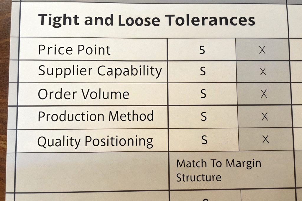
| Commercial Factor | Tight Tolerance Impact | Loose Tolerance Impact | Optimization Strategy |
|---|---|---|---|
| Price Point | 5-20% cost premium | 3-8% waste cost | Match to margin structure |
| Supplier Capability | Limits supplier options | Increases supply risk | Tiered supplier strategy |
| Order Volume | Higher initial cost, lower waste | Lower initial cost, higher waste | Volume-dependent tolerance |
| Production Method | Automated cutting requires precision | Manual cutting accommodates variation | Technology-appropriate standards |
| Quality Positioning | Brand equity protection | Potential reputation damage | Alignment with brand promise |
A global retailer optimized their tolerance strategy by implementing three tiers: luxury lines (tight tolerances, premium pricing), core lines (commercial tolerances, competitive pricing), and value lines (wider tolerances, cost leadership). This segmented approach to commercially-optimized tolerance setting maximized overall profitability.
How does supplier relationship affect tolerance negotiation?
Supplier relationship significantly impacts tolerance negotiation through trust, communication, and shared improvement objectives. Long-term partnerships typically achieve 20-30% tighter tolerances than transactional relationships through joint process improvement and better understanding of requirements.
We've quantified the relationship impact:
| Relationship Level | Typical Tolerance Achievement | Improvement Mechanisms |
|---|---|---|
| Transactional | Commercial standards | Limited communication, price focus |
| Preferred Supplier | 10-15% improvement vs. transactional | Regular feedback, basic collaboration |
| Strategic Partner | 20-30% improvement vs. transactional | Joint development, transparency, investment sharing |
| Vertical Integration | 30-50% improvement vs. transactional | Complete control, aligned objectives |
A Danish fashion brand achieved exceptional consistency by developing their key mill's capabilities—their investment in technical training and process improvement yielded 25% tighter tolerances without price increases. This collaborative approach to supplier capability development creates mutual benefit.
What testing frequency ensures compliance without excessive cost?
Testing frequency must provide sufficient confidence in compliance while minimizing costs that can reach $100-500 per test for comprehensive evaluation. Statistical sampling based on production volume and process stability typically provides optimal balance, with increased frequency for new suppliers or unstable processes.
Our testing frequency guidelines balance risk and cost:
| Risk Level | Recommended Sampling | Typical Cost Impact | Compliance Confidence |
|---|---|---|---|
| New Supplier/Process | 100% first lot, then 30% | 0.8-1.2% of order value | 99%+ |
| Established Stable Process | 10-15% of lots | 0.2-0.4% of order value | 95-98% |
| High-Volume Production | Statistical (AQL based) | 0.1-0.2% of order value | 90-95% |
| Critical Applications | 100% testing | 1.5-2.5% of order value | 99.9%+ |
| Low Risk/Value Items | Spot checking (2-5%) | <0.1% of order value | 80-85% |
An American uniform company optimized their testing costs by implementing risk-based sampling—their $1.2 million testing budget was reduced by 35% while maintaining equivalent quality assurance through better statistical methods. This data-driven approach to testing frequency optimization maximizes resource allocation.
Conclusion
Setting appropriate tolerances for GSM, width, and shade requires balancing technical feasibility, commercial requirements, and relationship considerations. The most effective approach involves setting tiered tolerances based on product positioning, implementing clear measurement protocols, establishing statistical sampling plans, and developing supplier capabilities through collaborative relationships.
Through establishing tolerance standards for diverse global brands, we've consistently found that the optimal approach combines technical understanding with commercial pragmatism. The most successful companies implement clear, achievable tolerances that suppliers can consistently meet, rather than theoretical ideals that create constant disputes and supply chain disruptions.
If you're developing tolerance specifications for your purchase orders, contact our Business Director Elaine at elaine@fumaoclothing.com. We'll share our comprehensive tolerance database and help you establish standards that balance technical requirements, commercial realities, and supply chain capabilities. With our vertical manufacturing experience, we can provide practical guidance on achievable tolerances across fabric types and manufacturing technologies.